Linearization of sensor characteristics

Linearization of sensor characteristics — a non-linear transformation of the sensor output value or a quantity proportional to it (analog or digital) that achieves a linear relationship between the measured value and the value representing it.

With the help of linearization, it is possible to achieve linearity on the scale of the secondary device to which a sensor with a non-linear characteristic is connected (eg thermocouple, thermal resistance, gas analyzer, flow meter, etc.). The linearization of the sensor characteristics makes it possible to obtain the necessary measurement accuracy through secondary devices with a digital output. This is necessary in some cases when connecting sensors to recording devices or when performing mathematical operations on the measured value (eg integration).

In terms of the encoder characteristic, the linearization acts as an inverse functional transformation.If the characteristic of the sensor is represented as y = F (a + bx), where x is the measured value, a and b are constants, then the characteristic of the linearizer connected in series with the sensor (Fig. 1) should look like this: z = kF (y), where F is the inverse function of F.

As a result, the output of the linearizer will be z = kF(F (a + bx)) = a ' + b'x, i.e. a linear function of the measured value.

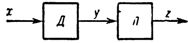
Rice. 1. Generalized linearization block diagram: D — sensor, L — linearizer.

Furthermore, by scaling, the dependence z is reduced to the form z '= mx, where m is the appropriate scale factor. If the linearization is done in a compensatory way, i.e. based on a servo system like Fig. 2, then the characteristic of the linearizing function converter should be similar to the characteristic of the sensor z = cF (a + bx), because the linearized value of the measured value is taken from the input of the converter of the function linearizer and its output is compared with the output value of the sensor.

A characteristic feature of linearizers as functional converters is a relatively narrow class of dependencies reproduced by them, limited to monotonic functions, which is determined by the type of sensor characteristics.

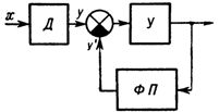
Rice. 2. Block diagram of linearization based on the tracking system: D — sensor, U — amplifier (transducer), FP — functional converter.

Linearizers can be classified according to the following criteria:

1. According to the method of setting the function: spatial in the form of templates, matrices, etc., in the form of a combination of non-linear elements, in the form of a digital calculation algorithm, devices.

2.By the degree of flexibility of the scheme: universal (ie, reconfigurable) and specialized.

3. By the nature of the structural diagram: open (Fig. 1) and compensation (Fig. 2) type.

4. In the form of input and output values: analog, digital, mixed (analog-digital and digital-analog).

5. By type of elements used in the circuit: mechanical, electromechanical, magnetic, electronic, etc.

Spatial function linearizers primarily include cam mechanisms, patterns, and non-linear potentiometers. They are used in cases where the measured value of each conversion stage is presented in the form of mechanical movement (cams — for linearization of the characteristics of manometric and transformer sensors, models — in recorders, non-linear potentiometers — in potential and bridge circuits).

The nonlinearity of the potentiometer characteristics is achieved by winding on profiled frames and sectioning using the piecewise linear approximation method by maneuvering the sections with suitable resistances.

In a linearizer based on an electromechanical servo system of the potentiometric type using a non-linear potentiometer (Fig. 3), the linearized value appears as an angle of rotation or mechanical displacement. These linearizers are simple, versatile and widely used in centralized control systems.

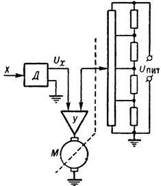
Rice. 3. Linearizer for electromechanical servo system of potentiometric type: D — sensor with output in the form of DC voltage, Y — amplifier, M — electric motor.

Non-linearities of the characteristics of individual elements (electronic, magnetic, thermal, etc.) are used in parametric functional converters. However, between the functional dependencies they develop and the characteristics of the sensors, it is usually not possible to achieve a complete match.

The algorithmic way of setting a function is used in digital function converters. Their advantages are high accuracy and stability of characteristics. They use the mathematical properties of individual functional dependencies or the principle of linear approximation by parts. For example, a parabola is developed based on the properties of squares of integers.

For example, a digital linearizer is based on the piecewise linear approximation method, which works on the principle of filling the approaching segments with pulses of different repetition rates. The filling frequencies change in jumps at the border points of the approaching segments according to the program inserted into the device according to the type of nonlinearity. The linearized quantity is then converted to a unitary code.

A partial linear approximation of the nonlinearity can also be performed using a digital linear interpolator. In this case, the filling frequencies of the interpolation intervals remain constant only on average.

The advantages of digital linearizers based on the method of linear approximation of parts are: ease of reconfiguration of the accumulated nonlinearity and the speed of switching from one nonlinearity to another, which is especially important in high-speed centralized control systems.

In complex control systems containing universal calculators, machines, linearization can be performed directly from these machines, in which the function is embedded in the form of a corresponding subroutine.