Flux and magnetic flux relationship

It is known from experience that near permanent magnets, as well as near current-carrying conductors, physical effects can be observed, such as mechanical impact on other magnets or current-carrying conductors, as well as the appearance of EMF in conductors moving in given space.

The unusual state of space near magnets and current-carrying conductors is called a magnetic field, the quantitative characteristics of which are easily determined by these phenomena: by the force of mechanical action or by electromagnetic induction, in fact, by the magnitude induced in a moving conductor EMF.

The phenomenon of conduction of EMF in the conductor (phenomenon of electromagnetic induction) occurs under different conditions. You can move a wire through a uniform magnetic field or simply change the magnetic field near a stationary wire. In either case, the change in the magnetic field in space will induce an EMF in the conductor.

A simple experimental device for investigating this phenomenon is shown in the figure. Here the conductive (copper) ring is connected with its own wires with a ballistic galvanometer, by the deflection of the arrow, for which it will be possible to estimate the amount of electric charge passing through this simple circuit. First, center the ring at some point in space near the magnet (position a), then move the ring sharply (to position b). The galvanometer will show the value of the charge passed through the circuit, Q.

Now we place the ring at another point, a little further from the magnet (to position c), and again, with the same speed, we move it sharply to the side (to position d). The deflection of the galvanometer needle will be less than in the first attempt. And if we increase the resistance of the loop R, for example, replacing copper with tungsten, then moving the ring in the same way, we will notice that the galvanometer will show an even smaller charge, but the value of this charge moving through the galvanometer in any case will be inversely proportional to the loop resistance.

The experiment clearly demonstrates that the space around the magnet at any point has some property, something that directly affects the amount of charge passing through the galvanometer when we move the ring away from the magnet. Let's call it something close to a magnet, magnetic flux, and we denote its quantitative value with the letter F. Note the revealed dependence of Ф ~ Q * R and Q ~ Ф / R.

Let's complicate the experiment. We will fix the copper loop at a certain point opposite the magnet, next to it (at position d), but now we will change the area of ​​the loop (overlapping part of it with a wire). The readings of the galvanometer will be proportional to the change in the area of ​​the ring (at position e).

Therefore, the magnetic flux F from our magnet acting on the loop is proportional to the area of ​​the loop. But the magnetic induction B, related to the position of the ring relative to the magnet, but independent of the parameters of the ring, determines the property of the magnetic field at any considered point in space near the magnet.

Continuing the experiments with a copper ring, we will now change the position of the plane of the ring relative to the magnet at the initial moment (position g) and then rotate it to a position along the axis of the magnet (position h).

Note that the greater the change in angle between the ring and the magnet, the more charge Q flows through the circuit through the galvanometer. This means that the magnetic flux through the ring is proportional to the cosine of the angle between the magnet and the normal to the plane of the ring.

Thus, we can conclude that magnetic induction B — there is a vector quantity, the direction of which at a given point coincides with the direction of the normal to the plane of the ring at that position when, when the ring is sharply moved away from the magnet, the charge Q passing along the circuit is maximum.

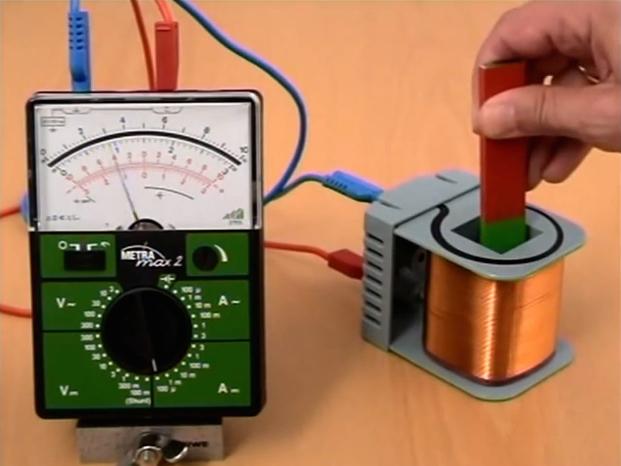
Instead of a magnet in the experiment you can use coil of an electromagnet, move this coil or change the current in it, thereby increasing or decreasing the magnetic field penetrating the experimental loop.

The area penetrated by the magnetic field cannot necessarily be bounded by a circular bend, it can in principle be any surface, the magnetic flux through which is then determined by integration:

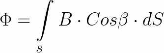
It turns out that magnetic flux F Whether the flux of the magnetic induction vector B through the surface S.And the magnetic induction B is the magnetic flux density F at a given point in the field. The magnetic flux Ф is measured in units of «Weber» — Wb. Magnetic induction B is measured in units of Tesla — Tesla.

If the entire space around a permanent magnet or a current-carrying coil is examined in a similar way, by means of a galvanometer coil, then it is possible to construct in this space an infinite number of the so-called "magnetic lines" — vector lines magnetic induction B — the direction of the tangents at each point of which will correspond to the direction of the magnetic induction vector B at these points of the studied space.

By dividing the space of the magnetic field by imaginary tubes with a unit cross-section S = 1, the so-called can be obtained. Single magnetic tubes whose axes are called single magnetic lines. Using this approach, you can visually depict a quantitative picture of the magnetic field, and in this case the magnetic flux will be equal to the number of lines passing through the selected surface.

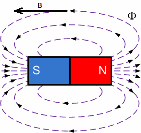
The magnetic lines are continuous, they leave the North Pole and necessarily enter the South Pole, so the total magnetic flux through any closed surface is zero. Mathematically it looks like this:

Consider a magnetic field bounded by the surface of a cylindrical coil. In fact, it is a magnetic flux that penetrates the surface formed by the turns of this coil. In this case, the total surface can be divided into separate surfaces for each of the turns of the coil. The figure shows that the surfaces of the upper and lower turns of the coil are pierced by four single magnetic lines, and the surfaces of the turns in the middle of the coil are pierced by eight.

To find the value of the total magnetic flux through all turns of the coil, it is necessary to sum the magnetic fluxes penetrating the surfaces of each of its turns, that is, the magnetic fluxes associated with the individual turns of the coil:

Ф = Ф1 + Ф2 + Ф3 + Ф4 + Ф5 + Ф6 + Ф7 + Ф8 if there are 8 turns in the coil.

For the symmetrical winding example shown in the previous figure:

F top turns = 4 + 4 + 6 + 8 = 22;

F lower turns = 4 + 4 + 6 + 8 = 22.

Ф total = Ф upper turns + Ф lower turns = 44.

This is where the concept of "flow connection" is introduced. Streaming connection The total magnetic flux associated with all turns of the coil, numerically equal to the sum of the magnetic fluxes associated with its individual turns:

Фm is the magnetic flux created by the current through one turn of the coil; wэ — effective number of turns in the coil;

The flux linkage is a virtual value because in reality there is no sum of individual magnetic fluxes, but there is a total magnetic flux. However, when the actual distribution of the magnetic flux over the turns of the coil is unknown, but the flux relation is known, then the coil can be replaced by an equivalent one by calculating the number of equivalent identical turns required to obtain the required amount of magnetic flux.