Impulse current

In various electronic devices, for example, in electronic and semiconductor equipment, i.e. in amplifiers, rectifiers, radios, generators, televisions, as well as in carbon microphones, telegraphs and many other devices, they are widely used ripple currents and voltages… In order not to repeat the reasoning twice, we will only talk about currents, but everything that is related to currents is also true for voltages.

Pulsating currents that have a constant direction but change their value can be different. Sometimes the current value changes from the highest to the lowest non-zero value. In other cases, the current is reduced to zero. If direct current circuit is interrupted at a certain frequency, then for some time intervals there is no current in the circuit.

In fig. 1 shows graphs of various wave currents. In fig. 1, a, b, the change in currents occurs according to sinusoidal curve, but these currents should not be considered sinusoidal alternating currents, since the direction (sign) of the current does not change. In fig.1, c shows a current consisting of separate pulses, that is, short-lived "shocks" of current, separated from each other by pauses of greater or lesser duration, and is often called pulsed current. Different pulsed currents differ from each other in the shape and duration of the pulses, as well as in the rate of repetition.

It is convenient to consider a pulsating current of any kind as the sum of two currents — direct and alternating, called term or component currents. Any pulsating current has DC and AC components. This seems strange to many. In fact, after all, a pulsating current is a current that flows all the time in one direction and changes its value.

How can you tell it contains alternating current that changes direction? However, if two currents — direct and alternating — pass simultaneously through the same wire, it turns out that a pulsating current will flow in that wire (Fig. 2). In this case, the amplitude of the alternating current should not exceed the value of the direct current. Direct and alternating currents cannot flow separately through the wire. They add to a general flow of electrons that has all the properties of a pulsating current.

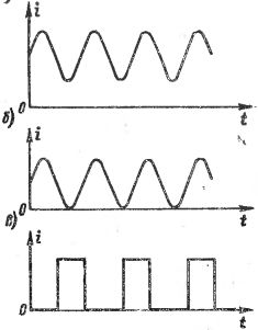
Rice. 1. Graphs of various wave currents

The addition of AC and DC currents can be shown graphically. In fig. 2 shows the graphs of a direct current equal to 15 mA and an alternating current with an amplitude of 10 mA. If we sum the values ​​of these currents for individual points in time, taking into account the directions (signs) of the currents, we get the wave current graph shown in fig. 2 with a bold line. This current varies from a low of 5 mA to a high of 25 mA.

The considered addition of currents confirms the validity of the representation of the pulsating current as a sum of direct and alternating currents. The correctness of this representation is also confirmed by the fact that with the help of some devices it is possible to separate the components of this current from each other.

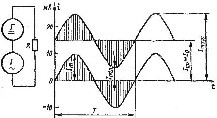
Rice. 2. Obtaining a pulsating current by adding direct and alternating current.

It should be emphasized that any current can always be represented as a sum of several currents. For example, a current of 5 A can be considered the sum of currents 2 and 3 A flowing in one direction, or the sum of currents 8 and 3 A flowing in different directions, that is, in other words, the difference between currents 8 and 3 A. It is not difficult to find other combinations of two or more currents giving a total of 5 A.

Here there is a complete similarity with the principle of addition and decomposition of forces. If two equally directed forces act on any object, they can be replaced by one common force. Forces acting in opposite directions can be replaced by a unit difference. Conversely, a given force can always be considered the sum of corresponding equally directed forces or the difference between oppositely directed forces.

It is not necessary to decompose direct or sinusoidal alternating currents into component currents. If we replace the pulsating current by the sum of direct and alternating currents, then by applying the known laws of direct and alternating currents to these component currents, it is possible to solve many problems and make the necessary calculations related to pulsating current.

The concept of pulsating current as a sum of direct and alternating currents is conventional.Of course, it cannot be assumed that at certain time intervals the direct and alternating currents really flow towards each other along the wire. In fact, there are no two opposite flows of electrons.

In reality, a pulsating current is a single current that changes its value over time. It is more correct to say that the pulsating voltage or pulsating EMF can be represented as the sum of the constant and variable components.

For example, in FIG. 2 shows how algebraically the constant emf of one generator is added to the variable emf of another generator. As a result, we have a pulsating EMF that causes the corresponding pulsating current. Conditionally, however, it can be considered that a constant EMF creates a direct current in the circuit, and an alternating EMF - an alternating current, which, when summed, forms a pulsating current.

Each pulsating current can be characterized by the maximum and minimum values ​​of Itax and Itin, as well as its constant and variable components. The constant component is denoted by I0. If the alternating component is a sinusoidal current, then its amplitude is denoted by It (all these quantities are shown in Fig. 2).

It should not be confused with It and Itax. Also, the maximum value of the current wave Imax should not be called the amplitude. The term amplitude usually refers only to alternating currents. Regarding the pulsating current, we can only talk about the amplitude of its variable component.

The constant component of the pulsating current can be called its average value Iav, that is, the arithmetic average value. Indeed, if we consider the changes in one period of the pulsating current shown in Fig.2, the following is clearly seen: in the first half-cycle, a number of values ​​are added to the 15 mA current by varying the current component, varying from 0 to 10 mA and back to 0, and in the second half-cycle, exactly the same current values ​​are subtracted from the current 15 mA.

Therefore, the current of 15 mA is really the average value. Since current is the transfer of electric charges through the cross-section of the wire, then Iav is the value of such a direct current that in one period (or for a whole number of periods) carries the same amount of electricity as this pulsating current.

For sinusoidal alternating current, the value of Iav per period is zero because the amount of electricity passed through the cross-section of the conductor in one half-period is equal to the amount of electricity passing in the opposite direction during another half-period. On the graphs of currents showing the dependence of current i on time t, the amount of electricity carried by the current is expressed by the area of ​​​​the figure bounded by the current curve, since the amount of electricity is determined by the product that it .

For a sinusoidal current, the areas of the positive and negative half waves are equal. In the pulsating current shown in fig. 2, during the first half period the amount of electricity carried by the AC component is added to the amount of electricity carried by the current Iav (shaded area in the figure). And during the second half cycle, exactly the same amount of electricity is withdrawn. As a result, the same amount of electricity is transferred throughout the entire period as with a single direct current Iav, that is, the area of ​​the rectangle Iav T is equal to the area bounded by the wave current curve.

Thus, the constant component or the average value of the current is determined by the transfer of electric charges through the cross section of the wire.

The current equation shown in Fig. 2 should obviously be written in the following form:

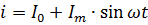
The power of the pulsating current must be calculated as the sum of the powers of its component currents. For example, if the current shown in Fig. 2, passes through a resistor of resistance R, then its power is

where I = 0.7Im is the rms value of the variable component.

You can introduce the concept of the rms value of the wave current Id. Power is calculated in the usual way:

Equating this expression to the previous one and reducing it with R, we get:

The same relationships can be obtained for stresses.