What is alternating current and how does it differ from direct current

Alternating current, In contrast DC current, is constantly changing both in magnitude and direction, and these changes occur periodically, that is, they repeat themselves at exactly equal intervals.

To induce such a current in the circuit, use alternating current sources that create an alternating EMF, periodically changing in magnitude and direction. Such sources are called alternators.

In fig. 1 shows a device diagram (model) of the simplest alternator. 

A rectangular frame made of copper wire, fixed on the axis and rotated in the field using a belt drive magnet… The ends of the frame are soldered to copper rings, which, rotating with the frame, slide on the contact plates (brushes).

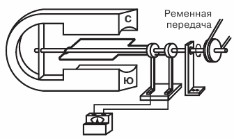
Figure 1. Diagram of the simplest alternator

Let's make sure that such a device is really a source of variable EMF.

Suppose a magnet creates between its poles uniform magnetic field, that is, one in which the density of magnetic field lines in each part of the field is the same.rotating, the frame crosses the lines of force of the magnetic field in each of its sides a and b EMF induced. 

Sides c and d of the frame do not work, because when the frame rotates, they do not cross the lines of force of the magnetic field and therefore do not participate in the creation of the EMF.

At any instant of time, the EMF occurring in side a is opposite in direction to the EMF occurring in side b, but in the frame both EMFs act according to and add to the total EMF, that is, induced by the entire frame.

This is easy to check if we use the right-hand rule we know to determine the direction of the EMF.

To do this, place the palm of the right hand so that it faces the north pole of the magnet, and the bent thumb coincides with the direction of movement of that side of the frame in which we want to determine the direction of the EMF. Then the direction of the EMF in it will be indicated by the outstretched fingers of the hand.

For whatever position of the frame we determine the direction of the EMF in sides a and b, they always add up and form a total EMF in the frame. At the same time, with each rotation of the frame, the direction of the total EMF in it changes to the opposite, since each of the working sides of the frame in one revolution passes under different poles of the magnet.

The magnitude of the EMF induced in the frame also changes as the rate at which the sides of the frame cross the magnetic field lines changes. Indeed, at the moment when the frame approaches its vertical position and passes it, the speed of crossing the lines of force on the sides of the frame is the highest, and the largest emf is induced in the frame.At those moments of time, when the frame passes its horizontal position, its sides seem to slide along the magnetic field lines without crossing them, and no EMF is induced.

Therefore, with uniform rotation of the frame, an EMF will be induced in it, periodically changing both in magnitude and direction.

The EMF occurring in the frame can be measured by a device and used to create a current in the external circuit.

Using phenomenon of electromagnetic induction, you can get alternating EMF and therefore alternating current.

Alternating current for industrial purposes and for lighting produced by powerful generators driven by steam or water turbines and internal combustion engines.

Graphic representation of AC and DC currents

The graphical method makes it possible to visualize the process of changing a certain variable depending on time.

Plotting variables that change over time begins by plotting two mutually perpendicular lines called the axes of the graph. Then, on the horizontal axis, on a certain scale, time intervals are plotted, and on the vertical axis, also on a certain scale, the values ​​of the quantity to be plotted (EMF, voltage or current).

In fig. 2 graphed direct current and alternating current ... In this case we delay the current values ​​and the current values ​​​​of one direction, which is usually called positive, are delayed vertically from the point of intersection of the axes O, and down from this point, the opposite direction, which is usually is called negative.

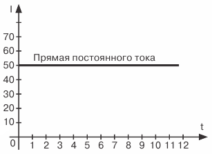
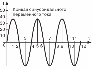Figure 2. Graphic representation of DC and AC

Point O itself serves both as the origin of current values ​​(vertically down and up) and time (horizontally right).In other words, this point corresponds to the zero value of the current and this starting point in time from which we intend to trace how the current will change in the future.

Let us verify the correctness of what is plotted in fig. 2 and a 50 mA DC current plot.

Since this current is constant, that is, it does not change its magnitude and direction over time, the same current values ​​will correspond to different moments of time, that is, 50 mA. Therefore, at the instant of time equal to zero, that is, at the initial moment of our observation of the current, it will be equal to 50 mA. Drawing a segment equal to the current value of 50 mA on the vertical axis upwards, we obtain the first point of our graph.

We must do the same for the next moment in time corresponding to point 1 on the time axis, that is, postpone from this point vertically upwards a segment also equal to 50 mA. The end of the segment will define the second point of the graph for us.

Having made a similar construction for several subsequent points in time, we obtain a series of points, the connection of which will give a straight line, which is a graphical representation of a constant current value of 50 mA.

Plotting a variable EMF

Let's move on to study variable graph of EMF... In fig. 3, a frame rotating in a magnetic field is shown at the top, and a graphical representation of the resulting variable EMF is given below.

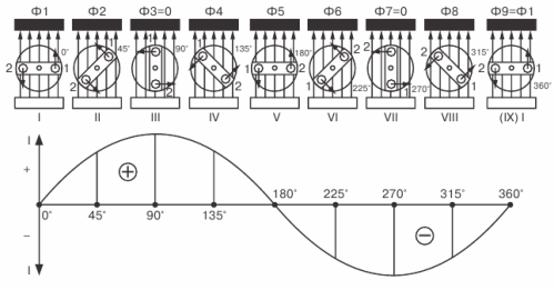Figure 3. Plotting the variable EMF

We begin to uniformly rotate the frame clockwise and follow the course of EMF changes in it, taking the horizontal position of the frame as the initial moment.

At this initial moment, the EMF will be zero because the sides of the frame do not cross the magnetic field lines.On the graph, this zero value of EMF corresponding to the instant t = 0 is represented by point 1.

With further rotation of the frame, the EMF will begin to appear in it and will increase until the frame reaches its vertical position. On the graph, this increase in EMF will be represented by a smooth rising curve that reaches its peak (point 2).

As the frame approaches the horizontal position, the EMF in it will decrease and drop to zero. On the graph, this will be depicted as a falling smooth curve.

Therefore, during the time corresponding to half a revolution of the frame, the EMF in it was able to increase from zero to the maximum value and decrease to zero again (point 3).

With further rotation of the frame, the EMF will reappear in it and gradually increase in magnitude, but its direction will already change to the opposite, as can be seen by applying the right-hand rule.

The graph takes into account the change in the direction of the EMF, so that the curve representing the EMF crosses the time axis and now lies below that axis. The EMF increases again until the frame assumes a vertical position.

Then the EMF will begin to decrease and its value will become equal to zero when the frame returns to its original position after completing one complete revolution. On the graph, this will be expressed by the fact that the EMF curve, reaching its peak in the opposite direction (point 4), will then meet the time axis (point 5)

This completes one cycle of changing the EMF, but if you continue the rotation of the frame, the second cycle immediately begins, exactly repeating the first, which in turn will be followed by the third, then the fourth, and so on until we stop the rotation frame.

Thus, for each rotation of the frame, the EMF occurring in it completes a complete cycle of its change.

If the frame is closed to some external circuit, then an alternating current will flow through the circuit, the graph of which will look the same as the EMF graph.

The resulting waveform is called a sine wave, and the current, EMF, or voltage varying according to this law is called sinusoidal.

The curve itself is called a sinusoid because it is a graphical representation of a variable trigonometric quantity called sine.

The sinusoidal nature of the current change is the most common in electrical engineering, therefore, speaking of alternating current, in most cases they mean sinusoidal current.

To compare different alternating currents (EMFs and voltages), there are values ​​that characterize a certain current. These are called AC parameters.

Period, Amplitude, and Frequency — AC parameters

Alternating current is characterized by two parameters — monthly cycle and amplitude, knowing which we can estimate what kind of alternating current it is and build a graph of the current.

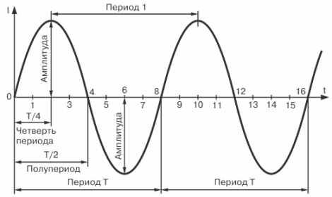
Figure 4. Sinusoidal current curve

The period of time during which a complete cycle of current change occurs is called a period. The period is denoted by the letter T and is measured in seconds.

The period of time during which half of a complete cycle of current change occurs is called a half cycle. Therefore, the period of change of current (EMF or voltage) consists of two half periods. It is quite obvious that all periods of the same alternating current are equal to each other.

As can be seen from the graph, during one period of its change, the current reaches twice its maximum value.

The maximum value of an alternating current (EMF or voltage) is called its amplitude or peak current value.

Im, Em, and Um are common designations for current, EMF, and voltage amplitudes.

First of all, we paid attention peak current, however, as can be seen from the graph, there are countless intermediate values ​​that are smaller than the amplitude.

The value of alternating current (EMF, voltage) corresponding to any selected moment in time is called its instantaneous value.

i, e and u are commonly accepted designations of the instantaneous values ​​of current, emf and voltage.

The instantaneous value of the current, as well as its peak value, is easy to determine with the help of the graph. To do this, from any point on the horizontal axis corresponding to the point in time we are interested in, draw a vertical line to the point of intersection with the current curve; the resulting segment of the vertical line will determine the value of the current at a given time, that is, its instantaneous value.

Obviously, the instantaneous value of the current after time T / 2 from the starting point of the graph will be zero, and after time T / 4 its amplitude value. The current also reaches its peak value; but already in the opposite direction, after a time equal to 3/4 T.

So the graph shows how the current in the circuit changes over time and that only one particular value of both the magnitude and direction of the current corresponds to each instant of time. In this case, the value of the current at a given point in time at one point in the circuit will be exactly the same at any other point in that circuit.

It is called the number of complete periods fulfilled by the current in 1 second of AC frequency and is denoted by the Latin letter f.

To determine the frequency of an alternating current, that is, to find out how many periods of its change the current made in 1 second, it is necessary to divide 1 second by the time of one period f = 1 / T. Knowing the frequency of the alternating current, you can to determine the period: T = 1 / f

AC frequency it is measured in a unit called hertz.

If we have an alternating current whose frequency is equal to 1 hertz, then the period of such a current will be equal to 1 second. Conversely, if the period of change of the current is 1 second, then the frequency of such a current is 1 hertz.

So we've defined AC parameters—period, amplitude, and frequency—that allow you to distinguish between different AC currents, EMFs, and voltages, and plot their graphs when necessary.

When determining the resistance of various circuits to alternating current, use another auxiliary value characterizing alternating current, the so-called angular or angular frequency.

Circular frequency denoted related to frequency f by the ratio 2 pif

Let's explain this dependency. When plotting the variable EMF graph, we saw that one complete rotation of the frame results in a complete cycle of EMF change. In other words, for the frame to make one revolution, that is, to rotate 360 ​​°, it takes a time equal to one period, that is, T seconds. Then, in 1 second, the frame makes a 360 ° / T revolution. Therefore, 360 ° / T is the angle through which the frame rotates in 1 second, and expresses the speed of rotation of the frame, which is usually called angular or circular speed.

But since the period T is related to the frequency f by the ratio f = 1 / T, then the circular speed can also be expressed as a frequency and will be equal to 360 ° f.

So we concluded that 360 ° f. However, for the convenience of using the circular frequency for any calculations, the 360 ​​° angle corresponding to one revolution is replaced by a radial expression equal to 2pi radians, where pi = 3.14. So we finally get 2pif. Therefore, to determine the angular frequency of alternating current (EMF or voltage), you must multiply the frequency in hertz by a constant number 6.28.