Kirchhoff's laws - formulas and examples of use

Kirchhoff's laws establish the relationship between currents and voltages in branched electrical circuits of any type. Kirchhoff's laws are of particular importance in electrical engineering because of their versatility, as they are suitable for solving any electrical problem. Kirchhoff's laws are valid for linear and non-linear circuits under constant and alternating voltage and current.

Kirchhoff's first law follows from the law of conservation of charge. It consists in the fact that the algebraic sum of currents converging in each node is equal to zero.

where is the number of currents merging at a given node. For example, for an electric circuit node (Fig. 1), the equation according to Kirchhoff's first law can be written in the form I1 — I2 + I3 — I4 + I5 = 0

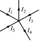
Rice. 1

In this equation, the currents directed into the node are assumed to be positive.

In physics, Kirchhoff's first law is the law of continuity of electric current.

Kirchhoff's second law: the algebraic sum of the voltage drop in individual sections of a closed circuit, arbitrarily chosen in a complex branched circuit, is equal to the algebraic sum of the EMF in this circuit

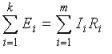
where k is the number of EMF sources; m- the number of branches in a closed loop; Ii, Ri- current and resistance of this branch.

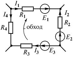
Rice. 2

So, for a closed-loop circuit (Fig. 2) E1 — E2 + E3 = I1R1 — I2R2 + I3R3 — I4R4

A note on the signs of the resulting equation:

1) EMF is positive if its direction coincides with the direction of arbitrarily selected circuit bypass;

2) the voltage drop in the resistor is positive if the direction of the current in it coincides with the direction of the bypass.

Physically, Kirchhoff's second law characterizes the balance of voltages in each circuit of the circuit.

Branch circuit calculation using Kirchhoff's laws

Kirchhoff's law method consists in solving a system of equations composed according to Kirchhoff's first and second laws.

The method consists in compiling equations according to Kirchhoff's first and second laws for the nodes and circuits of the electrical circuit and solving these equations in order to determine the unknown currents in the branches and, according to them, voltages. Therefore, the number of unknowns is equal to the number of branches, so the same number of independent equations must be formed according to Kirchhoff's first and second laws.

The number of equations that can be formed based on the first law is equal to the number of chain nodes, and only (y — 1) equations are independent of each other.

The independence of the equations is ensured by the choice of nodes. Typically, nodes are chosen such that each subsequent node differs from neighboring nodes by at least one branch.The remaining equations are formulated according to Kirchhoff's second law for independent circuits, i.e. number of equations b — (y — 1) = b — y +1.

A loop is called independent if it contains at least one branch that is not included in other loops.

Let's draw up a system of Kirchhoff equations for an electric circuit (Fig. 3). The diagram contains four nodes and six branches.

Therefore, according to Kirchhoff's first law, we compose y — 1 = 4 — 1 = 3equations, and to the second b — y + 1 = 6 — 4 + 1 = 3, also three equations.

We randomly choose the positive directions of the currents in all branches (Fig. 4). We choose the direction of passage of the contours clockwise.

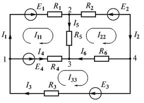
Rice. 3

We compose the required number of equations according to Kirchhoff's first and second laws

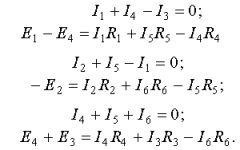
The resulting system of equations is solved with respect to the currents. If during the calculation the current in the branch turned out to be minus, then its direction is opposite to the assumed direction.

Potential Diagram — This is a graphical representation of Kirchhoff's second law that is used to check the correctness of calculations in linear resistive circuits. A potential diagram is drawn for a circuit without current sources, and the potentials of the points at the beginning and end of the diagram should be the same.

Consider the loop abcda of the circuit shown in fig. 4. In the branch ab between the resistor R1 and the EMF E1, we mark an additional point k.

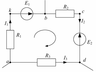
Rice. 4. Outline for building a potential diagram

The potential of each node is assumed to be zero (for example, ? a =0), choose the loop bypass and determine the potential of the loop points: ? a = 0 ,? k = ? a — I1R1, ?b =?k + E1 ,? c =?b — I2R2, ?d =? c -E2 ,?a =? d + I3R3 = 0

When constructing a potential diagram, it is necessary to take into account that the EMF resistance is zero (Fig. 5).

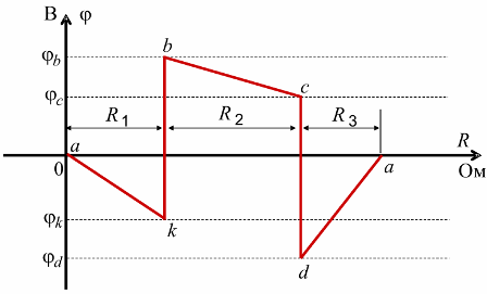
Rice. 5. Potential diagram

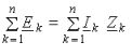
Kirchhoff's laws in complex form

For sinusoidal current circuits, Kirchhoff's laws are formulated in the same way as for direct current circuits, but only for complex values ​​of currents and voltages.

Kirchhoff's first law: «The algebraic sum of the complexes of the current in the node of the electric circuit is equal to zero»

Kirchhoff's second law: «In any closed circuit of an electrical circuit, the algebraic sum of the complex EMF is equal to the algebraic sum of the complex voltages on all passive elements of this circuit.»